The history of YOLO: The origin of the YOLOv1 algorithm

Real-time object detection tasks require both algorithmic accuracy and performance time in frames per second as much as possible, and most of the time, it's a trade-off between these metrics. So the YOLO algorithm and the zoo of its state-of-the-art modifications are a happy medium. Let's dive deep into the following:

• How it works
• Honest results
• Short overview of compared methods
• Positive in original YOLO
• Limitations and problems of YOLO
• Looks suspicious? Try it yourself!
• Further reading
• Key insights

How it works

In spite of the huge amount of YOLO algorithm implementations (seven evolution stages with several modifications per stage), key ideas are always the same:

1. Split the whole image into grid cells (using stacked convolutional layers).
2. For each cell, predict the boundary box.
3. Choose the best option (by coverage and confidence score) using probabilities, and voila!

Let's take a closer look.

The curse of the network

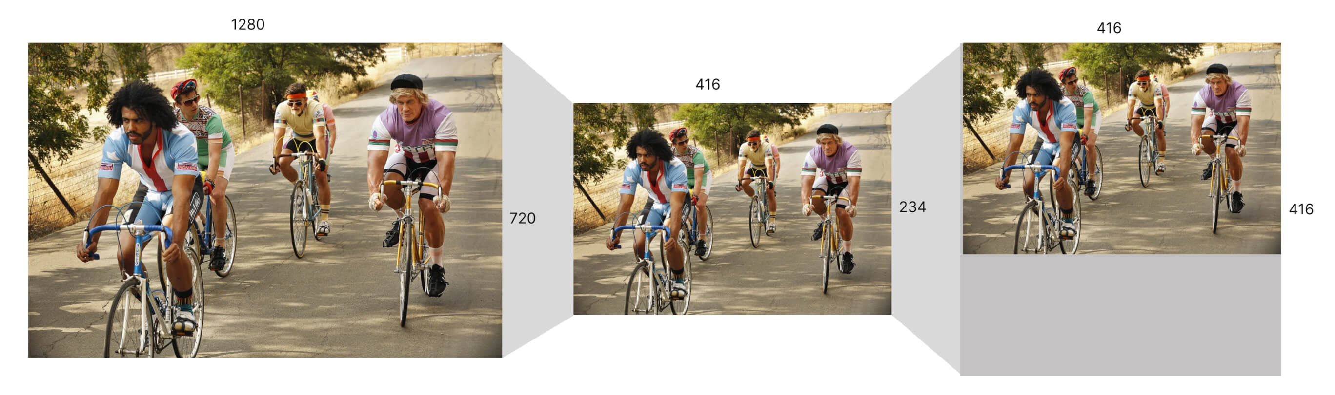
Just to make things clear: YOLO still has to resize the whole image (not like any sliding window methods, for example). For greater convenience, most of the implementations resize the whole image for you but be careful. The original YOLO implementation keeps the aspect ratio, i.e., the 1280×720 image will be resized to 416×234 and then will be inserted into the 416×416 network.

Is the grid all you need?

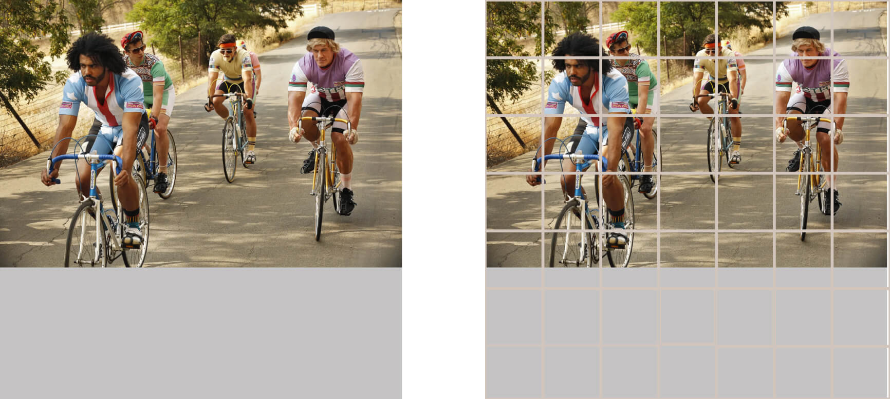
Let's split the entire image into S×S square cells of the same width and height (for example, the original algorithm uses a 7×7 grid). Then all future image manipulations will be only at a cellular level. At this point, you probably have at least two questions:

1. "Why do we need to use the grid cells?"

2. "Is seven a magic number?"

Let's start with question number two. The answer is: "No, seven is not a magic number." The square grid with 49 cells appears in the original article as constant for YOLO evaluation on the Pascal VOC dataset. And there is no proper research on how a particular grid cell size affects the detection quality and time (well, go ahead and do it yourself!) 💪.

The answer to question number one needs more explanation on the nature of the algorithm.

Regression is all you need!

Contrary to popular opinion, the most innovative idea behind the YOLO algorithms is to frame the object detection task as a regression problem (instead of repurposing classifiers to object detection, though let's discuss it later) and create a special architecture that can make both bounding box and class probability prediction.

So, what is the common way to solve object detection tasks? Let's check out R-CNN to simplify the explanation. According to a tech report by UC Berkeley, the simplest way to find objects on the entire image is… to find bounding boxes and classify them 😱. And the task of finding objects on an image can be defined as the regression task of predicting the (x,y) coordinates of the center and the (width, height) of object bounding boxes.

So, what have we learned so far about the YOLO object detection method? Well, for each cell, YOLO does the following:

1. Predicts bounding box coordinates, sizes for objects (two per cell for the original YOLO algorithm according to the original article), and their confidence scores — a measure of how likely it is for a cell to contain an object and how accurately we detect it.

2. Chooses only one predicted bounding box using confidence scores. 

3. Predicts conditional probabilities for each class (probabilities of whether the cell relates to a certain class when there is an object in it).

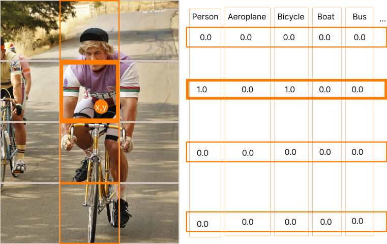
To get a clear understanding of how YOLO makes bounding box predictions let's check the "orange" grid cell on the picture above and the respective YOLO prediction:

1. The "orange" cell contains the center of the given bounding box (for example, a part of the detected object).

2. bx, by - center of the bounding box into the enveloping grid cell bounds (both coordinates should be in between the range [0.0, 1.0]).

3. bw, bh - bounding box width and height that are relative to the image width and height.

4. Confidence score (we will see how the confidence score prediction task is defined a little bit later).

For this current "orange" cell, the prediction value is (1.0, 0.8, 1.0, 1.5, 3.5), where the 1.0 value of the score means that there is definitely some object in the particular grid cell. In total, there are ten values for both bounding boxes.
So, YOLO authors treat object detection tasks as regression for spatially separated bounding boxes and associated class probabilities.

Intersection over Union threshold: The first step of filtering

The next step of the YOLO object detection algorithm is to manually filter bounding box predictions by confidence level with some threshold setting (usually, it's about 0.5).

So, where is the Intersection over Union (IoU) here? The answer is that the confidence level is the prediction of the IoU value with some ground truth box multiplied by the probability of whether a cell contains an object. More details about forming this prediction are in the neural network architecture and training section.

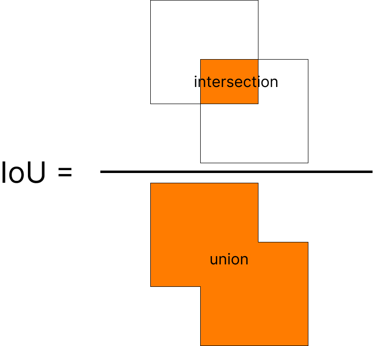
How is YOLO set up during the training process? What is the target? For a quick reminder of what IoU is, let's take a look at the image below.

def IOU(left_box, right_box):
    # lt - left top coords, rb - right bottom coords
    x1_lt, y1_lt,  x1_rb, y1_rb = left_box
    x2_lt, y2_lt,  x2_rb, y2_rb = right_box
    
    # coordinates of the area of intersection.
    i_x1 = max(x1_lt, x2_lt)
    i_y1 = max(y1_rb, y2_rb)
    i_x2 = max(x1_lt, x2_lt)
    i_y2 = max(x1_rb, x2_rb)

    i_height = max(i_y2 - i_y1 + 1, 0.0)
    i_width = max(i_x2 - i_x1 + 1, 0.)
     
    area_of_intersection = i_height * i_width

    # left width, height
    height1 = y1_lt - y1_rb + 1
    width1 = x1_rb - x1_lt + 1
     
    # right width, height
    height2 = y2_lt - y2_rb + 1
    width2 = x2_rb - x2_lt + 1
     
    area_of_union = height1 * width1 + height2 * width2 - area_of_intersection

    return area_of_intersection / area_of_union
   

Or you can just use torchvision.ops.box_iou instead.

import torch
from torchvision.ops import box_iou

box1 = torch.tensor([[511, 41, 577, 76]], dtype=torch.float)
box2 = torch.tensor([[544, 59, 610, 94]], dtype=torch.float)
iou = bops.box_iou(box1, box2)
# tensor([[0.1382]])

Check out our blog for a more detailed explanation of the Intersection over Union, one of the keystones in object detection.

So if our YOLO algorithm works perfectly, an ideal prediction (target) for a given cell (that contains the center of the given bounding box) will be:

1. If there is some object in the bounding box and we predict the bounding box perfectly.

2. If there is no object and we detect the absence.

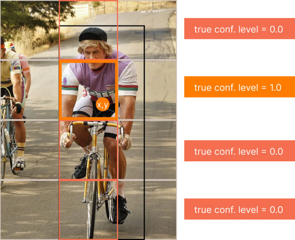
So, on the training step for the confidence level prediction task, for each cell, we put 1.0 if there is some object in the cell and the cell contains the center of the bounding box, and 0.0 if not.

This setup helps us pre-filter bounding boxes before the next step and will cost us O(Count of predictions). That helps us decrease the time of YOLO operation because the next step of filtering will cost us O(Count of prediction ^ 2).

Non-maximum Suppression: The final step of filtering

This is the final step of filtering bounding box candidates, so for one object, it will be only one bounding box. NMS algorithm uses B - list of bounding boxes candidates, C - list of their confidence values, and τ - the threshold for filtering overlapped bounding boxes. Let R be the result list:

1. Sort B according to their confidence scores in ascending order. 

2. Put the predicted box for B with the highest score (let it be a candidate) into R and remove it from B. 

3. Find all boxes from B with IoU(candidate, box) > τ and remove them from B. 

4. Repeat steps 1-3 until B is not empty.

def nms(boxes, confidences, overlapping_treshold):
    indexes = [i_s[0] for i_s in sorted(list(enumerate(confidences)), key=lambda v: v[1], reverse=True))
    boxes = [boxes[index_score[0]] for index_score in indexes]
    result = []
    while len(boxes) > 0:
        result.append(boxes.pop(0))
        removing_indexes = [i for i, box in enumerate(boxes) if IOU(box, result[-1]) >= overlapping_treshold]
        for index in removing_indexes:
            del boxes[index]

    return result
    

Or you can just use torchvision.ops.nms.

from torchvision.ops import nms

boxes = torch.tensor([[511, 41, 577, 76], [544, 59, 610, 94]], dtype=torch.float)
scores = torch.tensor([1.0, 0.5], dtype=torch.float])
overlapping_treshold = 0.5

result = nms(boxes, scores, overlapping_treshold)

Just because we have already filtered some trash on the previous step, this step doesn't cost much for YOLO (not like for R-CNN or DPM), but according to the original article from Darknet, it adds us about 2-3% in the final mean average precision (mAP).

What about the loss function?

So, as we already know, each YOLO grid cell predicts bounding boxes, confidence scores, and probability of classes. And the loss function contains all these tasks:

1. Object detection loss function - sum squared error of predicting center coordinates and the square root of bounding box width and height:

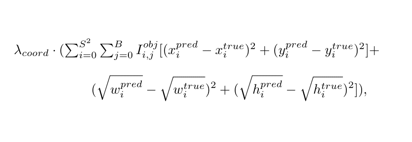
Where S is the count of rows in the grid, λ(coord) is the importance weight of the object detection task, I(obj, i, j) is the indicator value which denotes that ith (left to right, top to bottom) cell is responsible for the prediction of the bounding box with index j.

Why does the YOLO loss function use the square root for w, h? We are trying to use the same "dimension" for each part of the function.

2. Confidence prediction loss function - sum squared error of confidence levels for each pair of the box and grid cell.

As we try to predict the Intersection over Union (IoU) value with some ground truth box multiplied by the probability of containing an object in a grid cell (see Intersection over Union threshold: the first step of filtering), we may face a class imbalance problem, because most of the boxes don't contain any objects. The cure is that we can split the loss function into two parts: for a cell with and without a box. And then somehow decrease the weight of the cells without boxes.

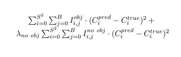
Where I(no obj, i, j) = 1 - I(obj, i, j), λ(no obj) is the weight for cells without any box (in the original article, it's 0.5).

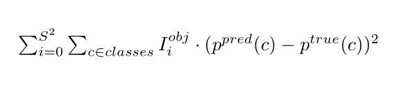
3. Classification loss function - sum squared error (yes, again) of each class probability for each cell.

Which neural network architecture can deal with it?

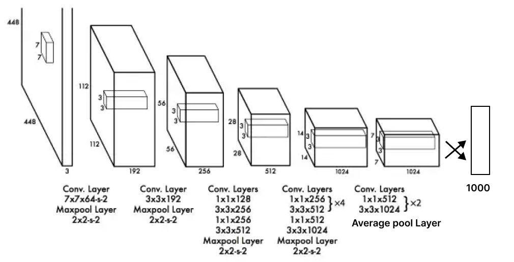
So, first of all 24 convolutional layers that "stretch" an image with size (448x448x3: w,h, RGB channels) into a tensor with the size of (SxSx1024, where S=7).  

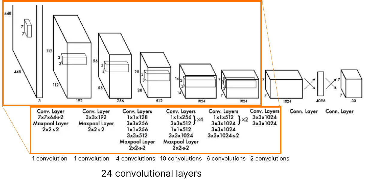
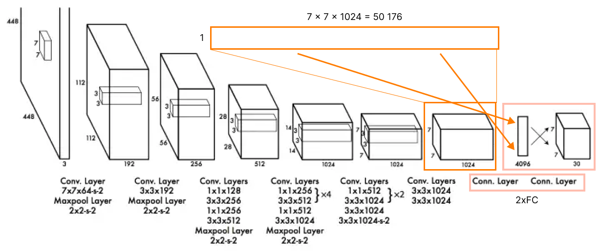
Then, two fully connected layers at the end (4096, 7x7x30). The first FC layer gets a flattened result of the last convolutional layer (7x7x1023 - 50176).

Each layer has Leaky ReLU as an activation function under the hood, except the final one, which uses the Linear activation function.

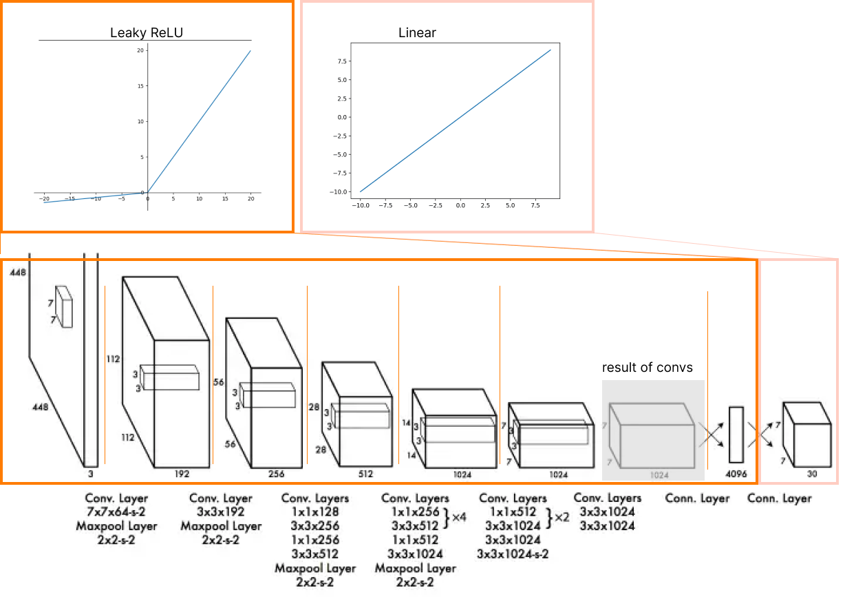
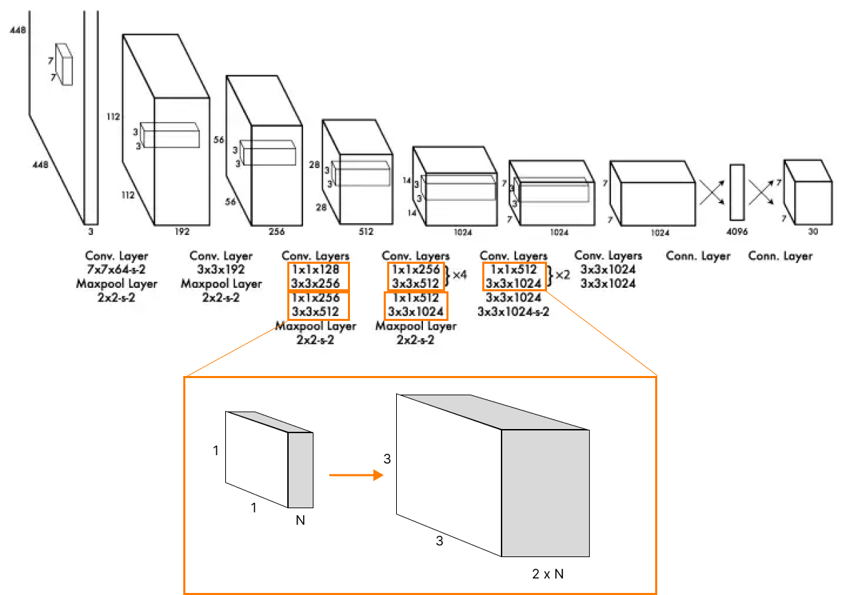
Instead of the inception modules used by GoogLeNet, YOLO architecture simply uses 1 × 1 reduction layers followed by 3 × 3 convolutions, similar to Lin's, Chen's, and Yan's Network in the network. More details are here.

To be honest, the last sentence is completely crtl+c - ctrl+v from the original article. There is no proper explanation of the intuition for such a method or a trick for less technically savvy folks (and for savvy too). Let's try to understand it together.

First of all, the main reason for stacking convolutional layers is always to extract features from some spatial structure of a given object (image, for most computer vision tasks).

And the main problem is that the “convolution queue” doesn't increase the degree of nonlinearity in the data structure. If you simply try to add some fully connected layers in between the convolutional blocks, it will absolutely destroy the spatial structure. And moreover, it will take more memory for calculation.

The simple solution is to add some nonlinearities by using nonlinear activation functions between convolutional layers. And YOLO algorithms use ReLU for it (see the bullet point above).

The other solution was given to us by Lin et al., 2013 article, and it's a simple insight: 1x1 convolutions add local nonlinearities across the channel activation.

For example, one of the most famous convolutional neural networks GoogleNet adds some kind of nonlinearities by using a block that stacks different convolutional representations of tensor: 1x1, 3x3, 5x5, and the tensor itself. And it's fine, but it takes a lot of RAM/VRAM memory for training and for inference.

But we are not Google, and moreover, we want to reach extremely fast performance (more frames per second, less inference speed 🔥) for the real-time object detection task even on mobile devices (for example, modern smartphones have about 6GB of RAM).

And 3x3 convolution "stretches" and "reduces" a spatial representation of the input image after the 1x1 convolutional stage. So, it decreases the width and height of tensors (each side lost 2 "pixels") and increases the count of channels two times.

And, of course, YOLO algorithms use some regularization techniques, such as data augmentation and dropout, to prevent overfitting.

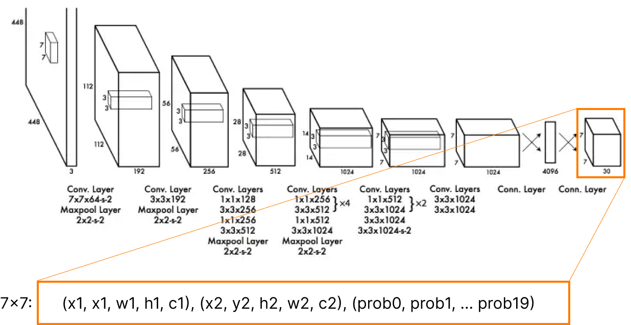
So the original YOLO model output for the Pascal VOC dataset has a 7x7x30 dimension, so it's (x,y,w,h,c) two times responsible for predicting objects and 20 class probabilities for each 49 "detectors."

What is the YOLO annotation format?

First, let's clarify it a bit: the YOLO architecture (and all future state-of-the-art models based on the idea) takes a single "look" at an input image to detect all objects on the grid. But in the training stage, you still need to prepare target data yourself. So, you need to:

• Resize the image
• Split the resized image into a grid
• And as we know, every cell is responsible for predicting a tensor of 30 values (for Pascal VOC object recognition task): (x,y,w,h,c) ×2 for the predicted bounding box, and 20 values of class probabilities. You need to prepare these values yourself.

For conditional class probabilities, it's all simple:

• The value is 1 if there is some object of the class in a cell, and this cell contains the center of the bounding box.
• In other cases, it's 0.

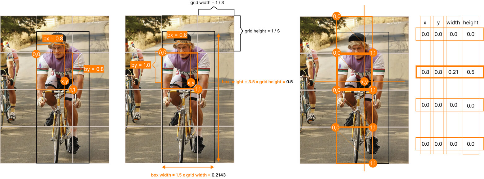
For bounding box coordinates, consider that the x,y center of the ground truth object should be set up according to the enveloping cell. So values x and y of the center should be in the range [0., 1.].

And you should set up the sizes of the bounding box relative to image sizes (416×416). Look at the picture above, instead of setting it (96, 224) in pixels, you should set it (0.2143, 0.5).

In the picture above, you can see the final result for the given bounding box for the "orange" cells.

Finally, let's explain again what is the confidence level target. In short, it's 1.0 if there is any object (its center, to be correct) in a given cell and 0.0 in other cases.

So, we have only two bounding boxes per cell, and it's completely up to you how two fill target data for each predictor. The main options and questions are:

• What is the priority value of using bounding boxes that have intersections?
• Which bounding box should be set as data for the first predictor? And which for the second?

So according to the original C++ code and YOLO as PyTorch library, the order is as follows: "which bounding box figures as the last in the line for an input image, that bounding box data fills target for both predictors."

You can use SuperAnnotate SDK to convert your YOLO data into SuperAnnotate format to fix annotation errors and label more data to improve your algorithm's average precision or accuracy.How to train this neural network.

How to train this neural network?

The first stage of the original training method of the first YOLO architecture is to prepare a pre-trained convolutional neural network.

For this purpose, Darknet decided to train the first 20 convolutional layers, followed by average pooling and fully connected layers for classification tasks on ImageNet 1000 classes data. According to the article, they achieve a single crop top-5 accuracy level of about 88% after the week of training.

Then they convert the pre-trained model to perform an object detection task (the pre-trained backbone is actually the so-called Darknet) in this way: inspired by the insight from Ren at. al article (Object detection networks on Convolutional Feature Maps) that adding both convolutional layers and fully connected layers to pre-trained image classification (and not only) networks can improve their performance values for object detection, they add four additional convolutional layers and two fully connected layers with randomly initialized weights.

Did they try a different configuration? We hope so, but we don't really know🤷‍♂️.

Training parameters can be different from task to task and from version to version, so we put together parameters and the training schedule from the original article for your own convenience:

• Training and validation data sets are Pascal VOC 2007 and 2012.
• About 135 epochs.
• Batch size: 64.
• Momentum: 0.9 | Decay: 0.0005.
• Learning rate: for the first epochs, slowly raise the learning rate from 1e−3 to 1e−2, continue training with 1e−2 for 75 epochs, then 1e−3 for 30 epochs, and finally 1e−4 for 30 epochs.
• The main insight is: if you start training a model on a high learning rate, the original YOLO will diverge due to unstable gradients.

Data augmentation:

• Random scaling and translations of up to 20% of the original image size.
• Random adjustment of the exposure and saturation of the image by up to a factor of 1.5 in the HSV color space.

So, finally, why do we use the grid?

Let's discuss another perspective: So, what is the alternative? Perhaps, we give N×(5 + C) predictions (where N - maximum of bounding boxes), and we can just add N units in a fully connected layer. But this leaves the network very "unconstrained." That means that we are likely to face a situation when the first 5 + C units specialize only in bicycle localization and others on detecting cars. Or the first 5 + C units specialize in left-side object recognition on the image, and others detect only the right side.

The reason you need a grid is to induce a bias that says, "these output units here are responsible for detecting objects in/on/covering exactly this region of the image."

Honest results

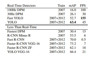
In brief, the original YOLO isn't good at detection quality compared to other object detection models (not-real time), even Fast R CNN. But the key point is that such methods are quite slow at inference (45 frames per second vs. 0.5). Though we can say that object detection models are actually real-time only if they achieve 30 frames per second or more.

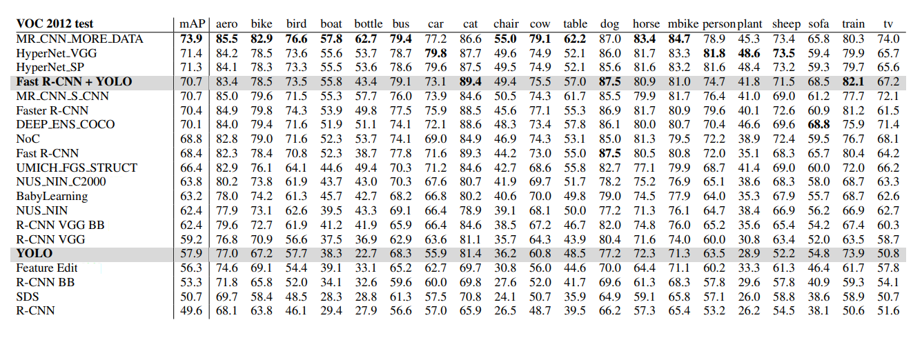
This is PASCAL VOC 2012 test dataset leaderboard, but again it's still not clear which datasets these models were trained on.

The most impressive moment in the YOLO algorithm is the achieved generalization. So, if we don't change the training data (again, it's different for Darknet and competitors) and get validation dataset from a completely different domain (for example, the Picasso Dataset and the People Art Dataset), and if we use the intersection between label classes, the results will be very impressive: So, I guess, it's not the merit of data augmentation 😅.

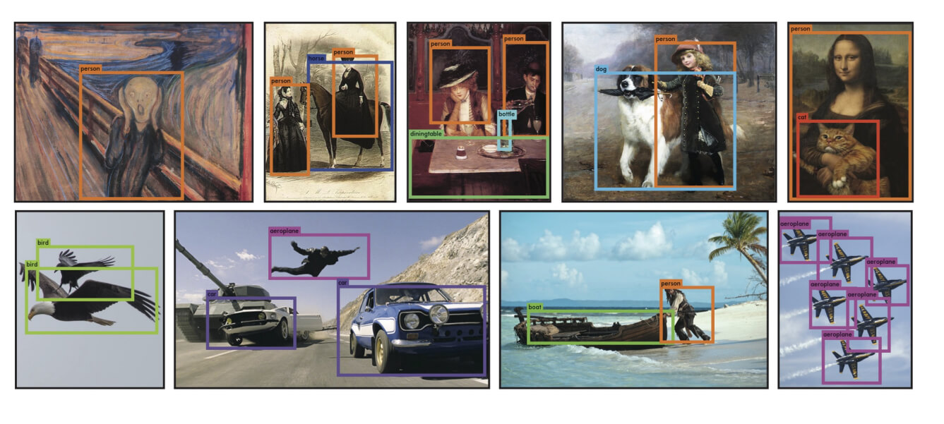
And if we use the intersection between label classes results will be very impressive:

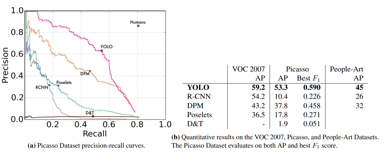
Well, I guess it's not the merit of data augmentation 😅.

Short overview of compared methods

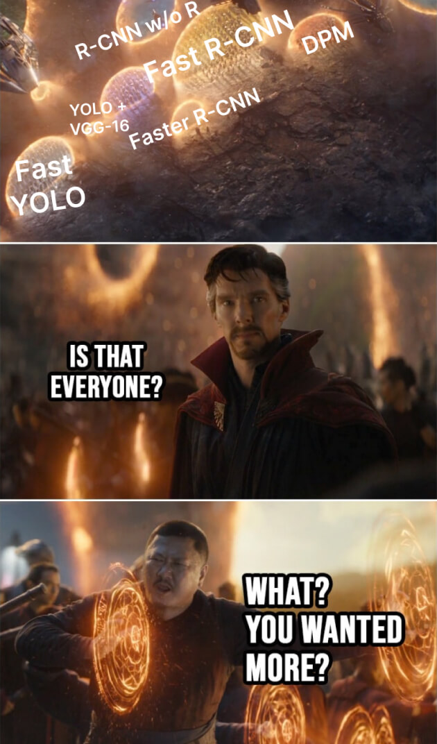
Let's quickly describe other detection methods that are mentioned in the original paper:

Region Proposals

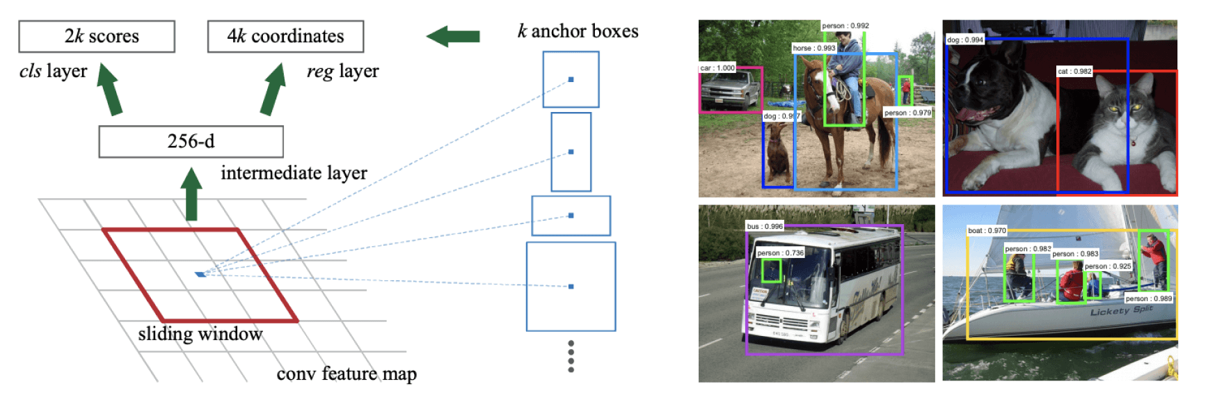
Competitors: R-CNN (Rich feature hierarchies for accurate object detection and semantic segmentation), Fast R-CNN (Original article with the same name), Faster R-CNN (Faster R-CNN: Towards Real-Time Object Detection with Region Proposal Networks).

Key ideas: predict region proposals using so-called anchor boxes (priors, manually predefined shapes) or so-called Selective Search, classify them as foreground (IoU with ground truth > 0.5) and background (IoU with ground truth < 0.1) using Support Vector Machine (for R-CNN) or single network (for Fast R-CNN) and then, try to adjust the chosen anchor boxes to ground truth shapes (predict shape shifts and object's center offset).

Key difference: Different networks for different steps (for example, Selective Search and then SVM) and slow resulting algorithm. YOLO uses a single convolutional neural network instead. By using constraints for grid cell detectors, YOLO gives much fewer proposals (only 98 per image compared to about 2000). It makes YOLO faster (18 frames per second maximum vs. 45 frames per second).

Deformable parts models

Competitors: Fastest DPM (The Fastest Deformable Part Model for Object Detection)

Key ideas: to use the window sliding approach or move on the picture with some smaller region, classify this region, and use high-scoring regions for object localization.

Key difference: YOLO performs object detection in a single stage (again) for all tasks, extracting features and detecting multiple objects and class probabilities directly while using the entire input image.

Deep convolutional networks

Competitors: VGG-16 (VERY DEEP CONVOLUTIONAL NETWORKS FOR LARGE-SCALE IMAGE RECOGNITION).

Key ideas: 16-weight convolutional layers and 3 fully connected layers. Large neural network? Not really, compared to 24 layers of YOLO. VGG-16 is used mostly for image classification tasks, but if you want to use it for object recognition, you need to change a head somehow.

Modifications and combinations

YOLO + VGG: So, Darknet guys did so; they used the VGG-16 feature extractor with the YOLO head.

Fast YOLO uses a neural network with fewer convolutional layers (9 instead of 24) and fewer filters in those layers. Other than the size of the network, all training and testing parameters are the same between YOLO and Fast YOLO.

Fast R-CNN + YOLO: for every predicted box by the R-CNN model, check to see if YOLO predicts a similar box, and if it does, give that prediction a boost based on the probability predicted by YOLO and the overlap between the two boxes.

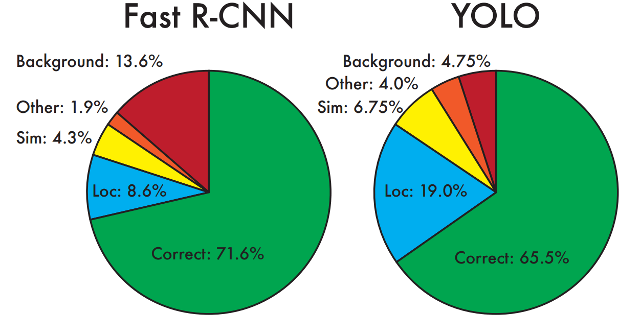
Key ideas: YOLO makes far fewer background mistakes than Fast R-CNN. By using YOLO to eliminate background detections from Fast R-CNN, we get a significant boost in detection performance.

Positive in original YOLO

Let's sum up the results:

• Quite accurate predictions for real-time object detection models using natural images.
• Quite good inference speed compared to some state-of-the-art (for that time) object detection architectures.
• Impressive generalizability: when R-CNN algorithms have a huge drop in average precision within the domain shift, the YOLO algorithm's average precision drops slightly.
• Fewer background errors compared to the Fast R-CNN algorithm (4.75% vs. 13.6%).

Limitations and problems of YOLO

Finally, let's sum up the problems and future areas for improvement:

• Each grid cell is responsible for the prediction of two boxes and can have only two classes
• YOLO is pretty bad at predicting groups of small boxes
• YOLO breaks with predicting new, unusual shapes or unusual aspect ratio
• Large boxes matter the same as small boxes in errors calculation
• It's particularly impossible to find all the objects for natural images (according to two maximum two boxes per cell constraint)
• Unstable gradient in early stages of training
• No batch normalization at all
• YOLO trains the classifier with 224x224 images and then moves to 448x448 images for object detection

Looks suspicious? Try it yourself!

There is an easy way to detect objects and touch the original YOLOv1 algorithm (spoiler: not actually).

Clone Darknet github repo:

git clone https://github.com/pjreddie/darknet.git

Compile the darknet binary file:

cd ./darknet
make -j2 .

Download the original YOLO weights file:

wget https://pjreddie.com/media/files/yolov1.weights

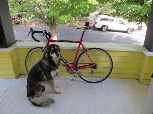
Darknet authors provide some test data as .jpg natural images located in ./darknet/data.

Use CLI to start the prediction (unfortunately, Darknet doesn't have any --help argument), and looks like it provides only per-image prediction:

./darknet detect ./cfg/yolov1.cfg ./yolov1.weights data/dog.jpg

The result of the prediction should appear at ./darknet/predictions.jpg. And unfortunately, it's not working as expected and does not predict anything at all (from scratch).

From the CLI output, we can notice that for this current input image, it predicts some training with a low confidence level.

Loading weights from ./yolov1.weights...Done!
data/dog.jpg: Predicted in 4.625505 seconds.
train: 55%

Let’s try again, but with other parameters:

./darknet yolo test ./cfg/yolov1.cfg ./yolov1.weights data/dog.jpg

Yes, darknet CLI is a little bit confusing (no manual, no help argument, and no documentation), but let’s take a look at confidence scores:

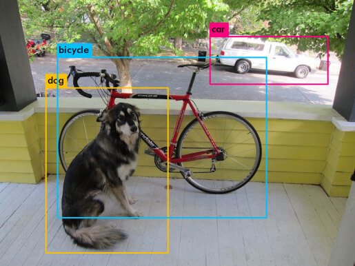
• data/dog.jpg: Predicted in 4.481968 seconds.
• dog: 26%
• car: 74%
• bicycle: 39%

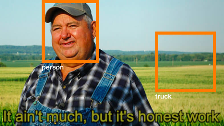
Looks like YOLO is not really sure about the dog and the bicycle. So, hope that the problem is the 59%-63% accuracy and I shouldn't throw my diploma into a trash bin. Let's try YOLOv3 (a spoiler for future articles).

wget https://pjreddie.com/media/files/yolov3.weights
./darknet detect ./cfg/yolov3.cfg ./yolov3.weights data/dog.jpg

Aaaaaaaand... it worked perfectly.

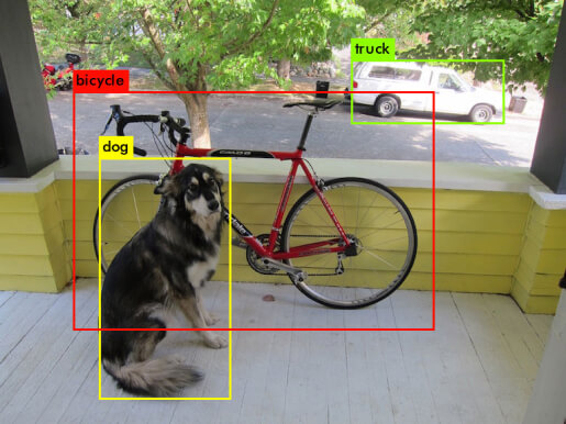
Loading weights from yolov3.weights...Done!

• data/dog.jpg: Predicted in 19.492208 seconds.
• dog: 100%
• truck: 92%
• bicycle: 99%

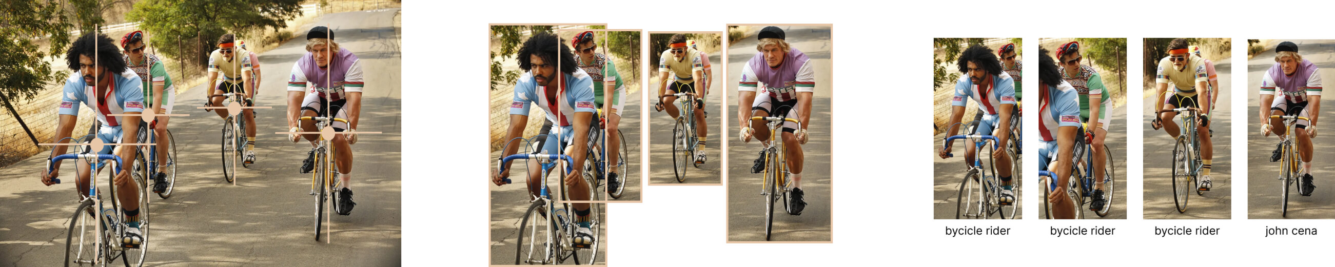
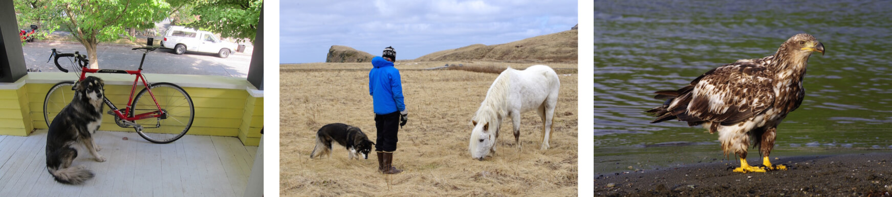
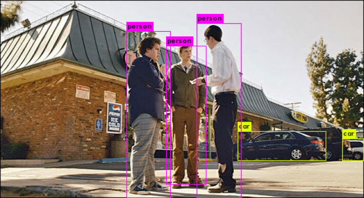
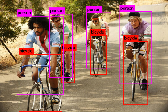
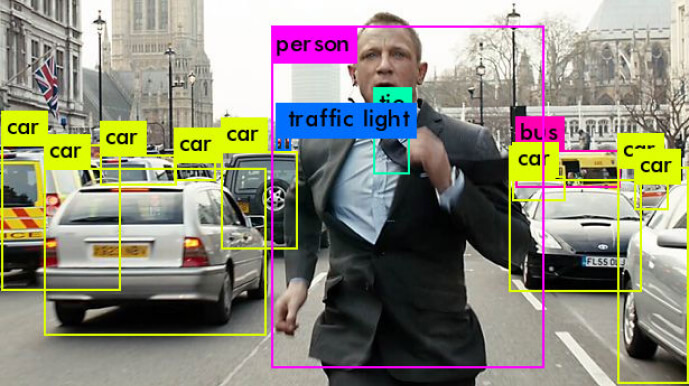
So let's try some out domain images, for example, some scenes from "SuperBad," "Tour de Pharmacy," and "Skyfall" movies.

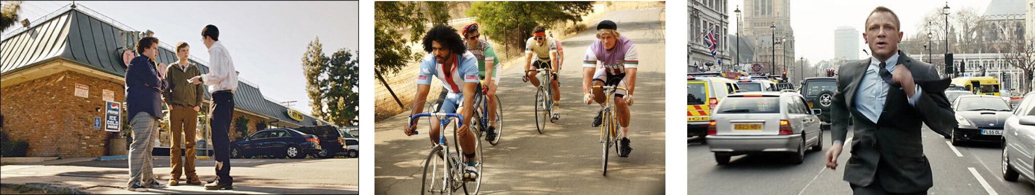
And it works pretty well too.

Let it be your treatment for reading the following articles about YOLO.

Further reading

Originally introduced by Joseph Redmon in 2015, Darknet, YOLO has sure come a long way. So, the plan is to create an ultimate guideline for each YOLO version, hope that there will be no new version of the YOLO model until we finish this overview.

Let's briefly check all the existing object detection YOLO versions as a teaser for the coming articles.

YOLOv2/YOLO9000: 2016, faster, better, stronger

Released in 2017, this version earned an honorable mention at CVPR 2017 because of significant improvements in anchor boxes and higher resolution. The main objective for YOLOv2 was to try and fix YOLO’s localization inaccuracy and inability to catch small objects in groups, as YOLO can only predict one object per grid cell. With YOLOv2, the user does not need to face such limitations because now it can predict several bounding boxes from a single cell.

YOLOv3: 2018, an incremental improvement

The 2018th release had an additional objectivity score to the bounding box prediction and connections to the backbone network layers. It also provided an improved performance on tiny objects because of the ability to run predictions at three different levels of granularity (see "feature pyramid network"). Although YOLOv2’s ability to predict bounding boxes (5 per cell) is higher than YOLOv3’s (3 per cell), YOLOv3 makes up for it by making those three predictions at different scales.

YOLOv4: 2020, optimal speed and accuracy of object detection

April's release of 2020 became the first paper not authored by Joseph Redmon. No matter how resourceful YOLOv3 was, similar to the previous algorithms, it still had shortcomings, which is why YOLOv4 was proposed. Here, Alexey Bochkovski introduced novel improvements, including mind activation, improved feature aggregation, etc. All of these improvements are achieved as a result of mixing YOLOv3’s training methods with the architectural layout modifications (for example, weighted residual connections).

YOLOv5: 2020, you don't need any paper if you have a good repo

Glenn Jocher continued to make further improvements in his June 2020 release, focusing on the architecture itself. YOLOv5 has four main models, namely (s) small, (m) medium, (l) large, and (x) extra large. Each of these models takes a different time to train, and their levels of detection performance and detection accuracy also differ.

It's honorable to mention that YOLOv5 has the best well-documented original repo.

YOLOv6: 2022, a single-stage object detection framework for industrial applications

Given that there was a two years gap, YOLOv6 authors tried to bring some bleeding edge techniques common for modern industry models like label assignment, self-distillation, more training epochs 🙃, quantization, and usage of RepVGG type backbone in network design.

YOLOv7: 2022, trainable bag-of-freebies sets new state-of-the-art real-time object detectors

This version of the YOLO algorithm shows us one of the highest average precision (about 56.8% on the MS COCO dataset) among all known real-time object detectors. The concept of the main modifications of YOLOv7 is complex enough not to be explained properly in 2-3 sentences, so we’ll take a closer look at this version of the YOLO algorithm in the coming articles.

YOLOv8: 2023, you don’t need any paper; part 2

Unfortunately, our “bad” expectations about releasing a new version of YOLO during editing this article came true. So, let me present to your attention another member of the YOLO family that has no published academic paper. But to be honest, the Ultralytics team did their best, and this version has the best documentation ever. 

Key insights

Despite YOLO’s utility in solving object detection issues, the algorithm still has several limitations; YOLO struggles in detecting minor details and small objects in an image, as each one of its grids can only detect one object and can only offer two bounding boxes per image. It is also important to mention that when compared to Faster R-CNN, YOLO has a relatively low recall rate and more localization errors.

The ongoing innovation will continue to generate more demand for computer vision models, where YOLO will still hold its special place for a number of reasons: YOLO heavily relies on a unified detection mechanism that consolidates different object detection elements into a single neural network to effectively perform computer vision tasks. Thanks to YOLO, the models can be trained with a single neural network into an entire detection pipeline.

It's not surprising that the algorithm found application in countless industries, eventually becoming the nexus for projects invested in object detection. Sounds like the right solution for your project? SuperAnnotate's end-to-end solution will eliminate the headache of annotating, training, and automating your AI. Feel free to explore further opportunities in our marketplace.